Isosurfaces with space group symmetry
Crystalline.jl implements a function levelsetlattice to generate symmetry-constrained periodic isosurfaces, following the approach described in Supplemental Section S3.D of Phys. Rev. X 12, 021066 (2022) which relates and constrains the orbits of an expansion in reciprocal-lattice plane waves.
The resulting isosurfaces can be visualized using a 3D-capable backend of Makie.jl such as GLMakie.jl.
Example
To illustrate the functionality, we construct and visualize an isosurface for the double gyroid in space group 230. First, we build a "base", unparameterized surface for space group 230:
julia> using Crystallinejulia> flat = levelsetlattice(230, Val(3))3-orbit Crystalline.UnityFourierLattice{3} [orbit-element (coefficient) …]: [[0,0,0] (1)] [[-2,-1,-1] (1), [-2,-1,1] (-1), [-2,1,-1] (1), [-2,1,1] (-1), [-1,-2,-1] (1), [-1,-2,1] (1), [-1,-1,-2] (1), [-1,-1,2] (-1), [-1,1,-2] (-1), [-1,1,2] (1), [-1,2,-1] (-1), [-1,2,1] (-1), [1,-2,-1] (-1), [1,-2,1] (-1), [1,-1,-2] (1), [1,-1,2] (-1), [1,1,-2] (-1), [1,1,2] (1), [1,2,-1] (1), [1,2,1] (1), [2,-1,-1] (-1), [2,-1,1] (1), [2,1,-1] (-1), [2,1,1] (1)] [[-2,-2,0] (1), [-2,0,-2] (1), [-2,0,2] (1), [-2,2,0] (1), [0,-2,2] (1), [0,2,-2] (1), [0,-2,-2] (1), [0,2,2] (1), [2,-2,0] (1), [2,0,-2] (1), [2,0,2] (1), [2,2,0] (1)]
By default, levelsetlattice returns a UnityFourierLattice, with the "joint" coefficient of each orbit set to unity. These coefficients can be freely chosen, however, with each choice of coefficients resulting in a different symmetry-respecting surface. Imposing a set of coefficients can be accomplished with modulate(flat, modulation), where modulation is a vector of orbit-coefficients (random, if unspecified), which multiplies onto the coefficients of each orbit.
julia> mflat = modulate(flat, [0, 1, 0.5])3-orbit ModulatedFourierLattice{3} [orbit-element (coefficient) …]:
 [[0,0,0] (0)]
 [[-2,-1,-1] (1), [-2,-1,1] (-1), [-2,1,-1] (1), [-2,1,1] (-1), [-1,-2,-1] (1), [-1,-2,1] (1), [-1,-1,-2] (1), [-1,-1,2] (-1), [-1,1,-2] (-1), [-1,1,2] (1), [-1,2,-1] (-1), [-1,2,1] (-1), [1,-2,-1] (-1), [1,-2,1] (-1), [1,-1,-2] (1), [1,-1,2] (-1), [1,1,-2] (-1), [1,1,2] (1), [1,2,-1] (1), [1,2,1] (1), [2,-1,-1] (-1), [2,-1,1] (1), [2,1,-1] (-1), [2,1,1] (1)]
 [[-2,-2,0] (0.5), [-2,0,-2] (0.5), [-2,0,2] (0.5), [-2,2,0] (0.5), [0,-2,2] (0.5), [0,2,-2] (0.5), [0,-2,-2] (0.5), [0,2,2] (0.5), [2,-2,0] (0.5), [2,0,-2] (0.5), [2,0,2] (0.5), [2,2,0] (0.5)]
The particular choice of modulation [0, 1, 0.5] above creates a double gyroid-like structure, but many other outcomes are possible, depending on the modulation. We can visualize the resulting structure using GLMakie.jl (for which we must also supply a set of basis vectors):
julia> using GLMakiejulia> Rs = directbasis(230, Val(3))DirectBasis{3} (cubic): [1.0, 0.0, 0.0] [0.0, 1.0, 0.0] [0.0, 0.0, 1.0]
plot(mflat, Rs; filling = 0.3)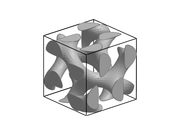
In the above, filling sets the filling fraction of the displayed lattice (see also filling2isoval and isoval2filling to map between filling fractions and isovalues).
By default, levelsetlattice (and directbasis) operates in the conventional basis. Conversion to a primitive basis (here, body-centered with centering type I) can be achieved via primitivize:
plot(primitivize(mflat, 'I'), primitivize(Rs, 'I'); filling = 0.3)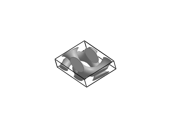
API
Crystalline.UnityFourierLattice — Type
UnityFourierLattice{D} <: AbstractFourierLattice{D}A general D-dimensional Fourier (plane wave) lattice specified by orbits of reciprocal lattice vectors (orbits) and coefficient interrelations (orbitcoefs)). The norm of all elements in orbitcoefs is unity. orbits (and associated coefficients) are sorted in order of increasing norm (low to high).
Crystalline.ModulatedFourierLattice — Type
ModulatedFourierLattice{D} <: AbstractFourierLattice{D}A D-dimensional concrete Fourier (plane wave) lattice, derived from a UnityFourierLattice{D} by scaling and modulating its orbit coefficients by complex numbers; in general, the coefficients do not have unit norm.
Crystalline.levelsetlattice — Function
levelsetlattice(sgnum::Integer, D::Integer=2, idxmax::NTuple=ntuple(i->2,D))
    --> UnityFourierLattice{D}
Compute a "neutral"/uninitialized Fourier lattice basis, a UnityFourierLattice, consistent with the symmetries of the space group sgnum in dimension D. The resulting lattice flat is expanded in a Fourier basis split into symmetry-derived orbits, with intra-orbit coefficients constrained by the symmetries of the space-group. The inter-orbit coefficients are, however, free and unconstrained.
The Fourier resolution along each reciprocal lattice vector is controlled by idxmax: e.g., if D = 2 and idxmax = (2, 3), the resulting Fourier lattice may contain reciprocal lattice vectors (k₁, k₂) with k₁∈[0,±1,±2] and k₂∈[0,±1,±2,±3], referred to a 𝐆-basis.
This "neutral" lattice can, and usually should, be subsequently modulated by modulate (which modulates the inter-orbit coefficients, which may eliminate "synthetic symmetries" that can exist in the "neutral" configuration, due to all inter-orbit coefficients being set to unity).
Examples
Compute a UnityFourierLattice, modulate it with random inter-orbit coefficients via modulate, and finally plot it (via Makie.jl):
julia> uflat = levelsetlattice(16, Val(2))
julia> flat  = modulate(uflat)
julia> Rs    = directbasis(16, Val(2))
julia> using GLMakie
julia> plot(flat, Rs)Crystalline.modulate — Function
modulate(flat::UnityFourierLattice{D},
modulation::AbstractVector{<:Number}=rand(ComplexF64, length(getcoefs(flat))),
expon::Union{Nothing, Real}=nothing, Gs::Union{ReciprocalBasis{D}, Nothing}=nothing)
                        --> ModulatedFourierLattice{D}
Derive a concrete, modulated Fourier lattice from a UnityFourierLattice flat (containing the interrelations between orbit coefficients), by multiplying the "normalized" orbit coefficients by a modulation, a complex modulating vector (in general, should be complex; otherwise restores unintended symmetry to the lattice). Distinct modulation vectors produce distinct realizations of the same lattice described by the original flat. By default, a random complex vector is used.
An exponent expon can be provided, which introduces a penalty term to short- wavelength features (i.e. high-|G| orbits) by dividing the orbit coefficients by |G|^expon; producing a "simpler" and "smoother" lattice boundary when expon > 0 (reverse for expon < 0). This basically amounts to a continuous "simplifying" operation on the lattice (it is not necessarily a smoothing operation; it simply suppresses "high-frequency" components). If expon = nothing, no rescaling is performed. If Gs is provided as nothing, the orbit norm is computed in the reciprocal lattice basis (and, so, may not strictly speaking be a norm if the lattice basis is not cartesian); to account for the basis explicitly, Gs must be provided as a ReciprocalBasis, see also normscale.
Crystalline.filling2isoval — Function
filling2isoval(
    flat::Crystalline.AbstractFourierLattice{D}
) -> Any
filling2isoval(
    flat::Crystalline.AbstractFourierLattice{D},
    filling::Real
) -> Any
filling2isoval(
    flat::Crystalline.AbstractFourierLattice{D},
    filling::Real,
    nsamples::Integer
) -> Any
Return the isovalue of flat such that the interior of the thusly defined levelset isosurface encloses a fraction filling of the unit cell.
The keyword argument nsamples specifies the grid-resolution used in evaluating this answer (via Statistics.jl's quantile).
Crystalline.isoval2filling — Function
isoval2filling(
    flat::Crystalline.AbstractFourierLattice{D},
    isoval::Real
) -> Any
isoval2filling(
    flat::Crystalline.AbstractFourierLattice{D},
    isoval::Real,
    nsamples::Integer
) -> Any
Return the filling fraction of the interior of the isosurface defined by flat for an isovalue isoval.
The keyword argument nsamples specifies the grid-resolution used in evaluating this answer (using staircase integration).
Bravais.primitivize — Method
primitivize(flat::AbstractFourierLattice, cntr::Char) --> ::typeof(flat)Given flat referred to a conventional basis with centering cntr, compute the derived (but physically equivalent) lattice flat′ referred to the associated primitive basis.
Specifically, if flat refers to a direct conventional basis Rs $≡ (\mathbf{a} \mathbf{b} \mathbf{c})$ [with coordinate vectors $\mathbf{r} ≡ (r_1, r_2, r_3)^{\mathrm{T}}$] then flat′ refers to a direct primitive basis Rs′ $≡ (\mathbf{a}' \mathbf{b}' \mathbf{c}') ≡ (\mathbf{a} \mathbf{b} \mathbf{c})\mathbf{P}$ [with coordinate vectors $\mathbf{r}' ≡ (r_1', r_2', r_3')^{\mathrm{T}} = \mathbf{P}^{-1}\mathbf{r}$], where $\mathbf{P}$ denotes the basis-change matrix obtained from primitivebasismatrix(...).
To compute the associated primitive basis vectors, see primitivize(::DirectBasis, ::Char) [specifically, Rs′ = primitivize(Rs, cntr)].
Examples
A centered ('c') lattice from plane group 5 in 2D, plotted in its conventional and primitive basis (requires a backend of Makie.jl, e.g., GLMakie.jl):
julia> sgnum = 5; D = 2; cntr = centering(sgnum, D)  # 'c' (body-centered)

julia> Rs   = directbasis(sgnum, Val(D))     # conventional basis (rectangular)
julia> flat = levelsetlattice(sgnum, Val(D)) # Fourier lattice in basis of Rs
julia> flat = modulate(flat)                 # modulate the lattice coefficients
julia> plot(flat, Rs)

julia> Rs′   = primitivize(Rs, cntr)    # primitive basis (oblique)
julia> flat′ = primitivize(flat, cntr)  # Fourier lattice in basis of Rs′

julia> using GLMakie
julia> plot(flat′, Rs′)Bravais.conventionalize — Method
conventionalize(flat::AbstractFourierLattice, cntr::Char) --> ::typeof(flat′)Given flat referred to a primitive basis with centering cntr, compute the derived (but physically equivalent) lattice flat′ referred to the associated conventional basis.
See also the complementary method primitivize(::AbstractFourierLattice, ::Char) for additional details.
Crystalline.AbstractFourierLattice — Method
(flat::AbstractFourierLattice)(xyz) --> Float64
(flat::AbstractFourierLattice)(xyzs...) --> Float64
Evaluate an AbstractFourierLattice at the point xyz and return its real part, i.e.
\[ \mathop{\mathrm{Re}}\sum_i c_i \exp(2\pi i\mathbf{G}_i\cdot\mathbf{r})\]
with $\mathrm{G}_i$ denoting reciprocal lattice vectors in the allowed orbits of flat, with $c_i$ denoting the associated coefficients (and $\mathbf{r} \equiv$ xyz).
xyz may be any iterable object with dimension matching flat consisting of real numbers (e.g., a Tuple, Vector, or SVector). Alternatively, the coordinates can be supplied individually (i.e., as flat(x, y, z)).